AI Tutorial: Learn PCA for STM32 TinyML. Optimize models using Python/scikit-learn & Iris data. Deploy with TFlite & X-Cube-AI.
Abstract
This article introduces Principal Component Analysis (PCA) as a powerful dimensionality reduction technique, highlighting its crucial role in optimizing machine learning models for resource-constrained embedded systems, specifically targeting STM32 microcontrollers. We’ll provide a Python-based hands-on example using the classic Iris dataset with scikit-learn, demonstrating how to apply PCA and use the reduced data for a simple classifier. Finally, we’ll discuss the essential role of tools like ONNX and TensorFlow Lite for Microcontrollers (TFlite) and ST’s X-Cube-AI in deploying these optimized models to the edge, using the Cloud Edge platform.
1. Introduction
Machine Learning (ML) is increasingly migrating from the cloud to the “edge”—devices like IoT sensors and microcontrollers. However, microcontrollers such as the STM32 family have limited Flash, RAM, and processing power. This presents a significant challenge for deploying complex ML models. Dimensionality reduction techniques like PCA are vital tools in the tinyML ecosystem. By reducing the number of input features while retaining most of the essential information, PCA helps decrease the model’s complexity, memory footprint, and inference time, making deployment feasible on resource-limited STM32 devices.
2. Prerequisites
For the Python Hands On section, you will need:
- Python 3.x
- scikit-learn: For PCA and classification.
- pandas and numpy: For data manipulation.
- matplotlib and seaborn: (Optional) For visualization.
For the embedded deployment discussion, general familiarity with STM32 microcontrollers and the STM32CubeMX environment is helpful.
- Several boards can be used, this article will focus on B-U585-IOT02A
3. Concepts
3.1 PCA
Principal Component Analysis (PCA) is an unsupervised, linear transformation technique used for dimensionality reduction. The goal is to project a high-dimensional dataset onto a lower-dimensional subspace such that the variance of the data in the new subspace is maximized.
- Principal Components: The new axes (Principal Components or PCs) are linear combinations of the original features. The first PC captures the maximum variance, the second PC captures the maximum remaining variance and is orthogonal to the first, and so on.
- Model Optimization: By selecting only the top few Principal Components, we significantly reduce the size of the input data vector. For an embedded system, this translates directly to:
- Reduced RAM/Flash usage: Smaller input vectors mean smaller feature buffers.
- Faster Inference: Fewer input values lead to fewer calculations in the subsequent classifier/neural network.
If the model is simple, the benefits provided by PCA usage will not outweigh its cost in memory usage and time to be executed. This is highly useful for images, but not that much for simpler cases, such as the IRIS dataset;
3.2 Classifier
After applying PCA, the reduced-dimension data can be used to train a classifier. The choice of classifier (e.g., K-Nearest Neighbors, Decision Tree, or a small Neural Network) depends on the specific STM32’s capabilities.
For tinyML applications, minimizing the model complexity is key, and the data compression provided by PCA helps the classifier maintain accuracy even with fewer training parameters.
The core idea is that the computationally expensive PCA transformation is done once during the model preparation phase, and only the resulting transformation matrix (eigenvectors) is stored on the STM32 to project new input data in real-time.
For this example, the classifier used is a simple Multi-Layer Perceptron (MLP) model from scikit-learn.
3.3 Multi-Layer Perceptron (MLP) Classifier
For this example, the classifier used is a simple Multi-Layer Perceptron (MLP) model from scikit-learn.
For tinyML applications, minimizing the model complexity is key. This simple Neural Network structure is highly efficient.
3.4 ONNX and TFlite and X-Cube-AI Usage
TensorFlow Lite for Microcontrollers (TFLite Micro) is an open-source library designed to run ML models on microcontrollers. To deploy a model that utilizes PCA on an STM32, the standard workflow often involves training a complete model (PCA + Classifier) in a desktop environment (like Python/scikit-learn or TensorFlow/Keras) or via online notebooks, such as Google Colab.
This trained model is then converted into the optimized format (.tflite). TFLite Micro’s runtime is designed to fit within the small memory footprint of microcontrollers, enabling on-device inference. STMicroelectronics also offers the X-Cube-AI tool, which often provides even greater optimization for STM32.
4. Hands On: PCA and Classification with Iris Dataset
The IRIS dataset is considered the “hello world” for AI, so we’ll use it as base for the article.
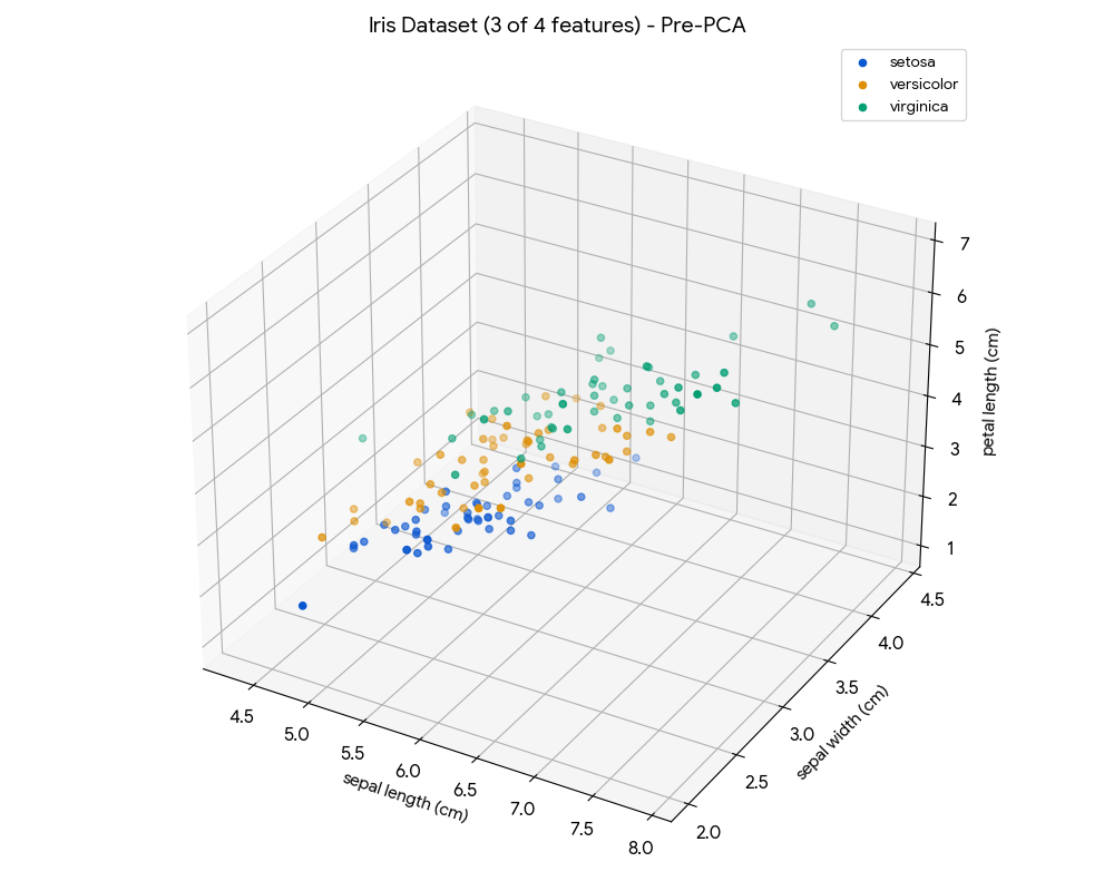
The Iris dataset contains four features (sepal length, sepal width, petal length, petal width) for 150 samples across three species. We will reduce this 4D problem to 2D using PCA for visualization and a basic classifier.
# -*- coding: utf-8 -*-
"""PCA_STM32.ipynb
Automatically generated by Colab.
Original file is located at
https://colab.research.google.com/drive/1uYlPi28C9nDe-cE2WTx2LwzbtbXfOlrj
"""
# --- External Libraries for Embedded Export (Requires pip install) ---
# import onnx
# from skl2onnx import convert_sklearn
# from skl2onnx.common.data_types import FloatTensorType
# from micromlgen import port
# ---------------------------------------------------------------------
pip install micromlgen
pip install skl2onnx
import pandas as pd
import numpy as np
import matplotlib.pyplot as plt
from mpl_toolkits.mplot3d import Axes3D
import seaborn as sns
from sklearn.datasets import load_iris
from sklearn.model_selection import train_test_split
from sklearn.preprocessing import StandardScaler
from sklearn.decomposition import PCA
from sklearn.neural_network import MLPClassifier
from sklearn.metrics import accuracy_score, confusion_matrix, ConfusionMatrixDisplay
# --- External Libraries for Embedded Export (Requires pip install) ---
import onnx
from skl2onnx import convert_sklearn
from skl2onnx.common.data_types import FloatTensorType
from micromlgen import port
# 1. Load Data
iris = load_iris()
X = iris.data
y = iris.target
feature_names = iris.feature_names
target_names = iris.target_names
# 2. Standardize the data (Crucial for PCA)
scaler = StandardScaler()
X_scaled = scaler.fit_transform(X)
# --- VISUALIZATION: 3D Plot BEFORE PCA (using 3 features) ---
fig = plt.figure(figsize=(10, 8))
ax = fig.add_subplot(111, projection='3d')
for i, target_name in enumerate(target_names):
ax.scatter(X[y == i, 0], X[y == i, 1], X[y == i, 2], label=target_name)
ax.set_xlabel(feature_names[0])
ax.set_ylabel(feature_names[1])
ax.set_zlabel(feature_names[2])
ax.set_title(f'Iris Dataset (3 of 4 features) - Pre-PCA')
ax.legend()
plt.tight_layout()
plt.show() # Display the plot
# -------------------------------------------------------------
# 3. Apply PCA: Reduce to 2 Principal Components (PC1 and PC2)
pca = PCA(n_components=2)
X_pca = pca.fit_transform(X_scaled)
# --- VISUALIZATION: 2D Plot AFTER PCA (PC1 and PC2) ---
pca_df = pd.DataFrame(data = X_pca, columns = ['principal component 1', 'principal component 2'])
pca_df['target'] = y
plt.figure(figsize=(8, 6))
target_names_list = [iris.target_names[i] for i in y]
sns.scatterplot(
x='principal component 1',
y='principal component 2',
hue=target_names_list,
palette=sns.color_palette("tab10", n_colors=3),
data=pca_df,
legend="full",
alpha=0.8
)
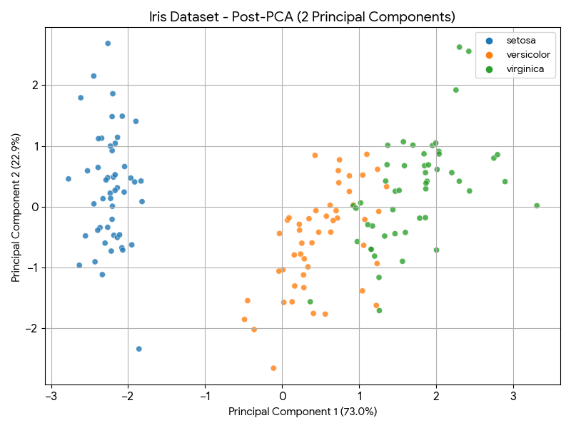
plt.title(f'Iris Dataset - Post-PCA (2 Principal Components)')
plt.xlabel(f'Principal Component 1 ({pca.explained_variance_ratio_[0]*100:.1f}%)')
plt.ylabel(f'Principal Component 2 ({pca.explained_variance_ratio_[1]*100:.1f}%)')
plt.grid()
plt.tight_layout()
plt.show() # Display the plot
# --------------------------------------------------------
# The PCA components (eigenvectors) are the core transformation matrix
# needed for real-time inference on the STM32.
# 4. Split Data (using the PCA-transformed data)
X_train, X_test, y_train, y_test = train_test_split(
X_pca, y, test_size=0.3, random_state=42, stratify=y
)
# 5. Train a Classifier (NEW: Simple Multi-Layer Perceptron/Neural Network)
# This is a small network suitable for embedded systems:
# - Hidden Layer 1: 10 neurons
# - Activation: ReLu (Rectified Linear Unit)
# - Max Iterations: 1000 (to ensure convergence)
mlp = MLPClassifier(
hidden_layer_sizes=(10,),
max_iter=1000,
activation='relu',
solver='adam',
random_state=42
)
mlp.fit(X_train, y_train)
# 6. Evaluate
y_pred = mlp.predict(X_test)
accuracy = accuracy_score(y_test, y_pred)
print("--- Results with Simple Neural Network (MLP) ---")
print(f"Classifier Accuracy (on 2D data): {accuracy:.4f}")
print(f"\nExplained Variance Ratio by the 2 Components: {pca.explained_variance_ratio_.sum():.4f}")
# --- VISUALIZATION: Confusion Matrix ---
cm = confusion_matrix(y_test, y_pred)
disp = ConfusionMatrixDisplay(confusion_matrix=cm, display_labels=target_names)
fig, ax = plt.subplots(figsize=(8, 8))
disp.plot(ax=ax, cmap=plt.cm.Blues)
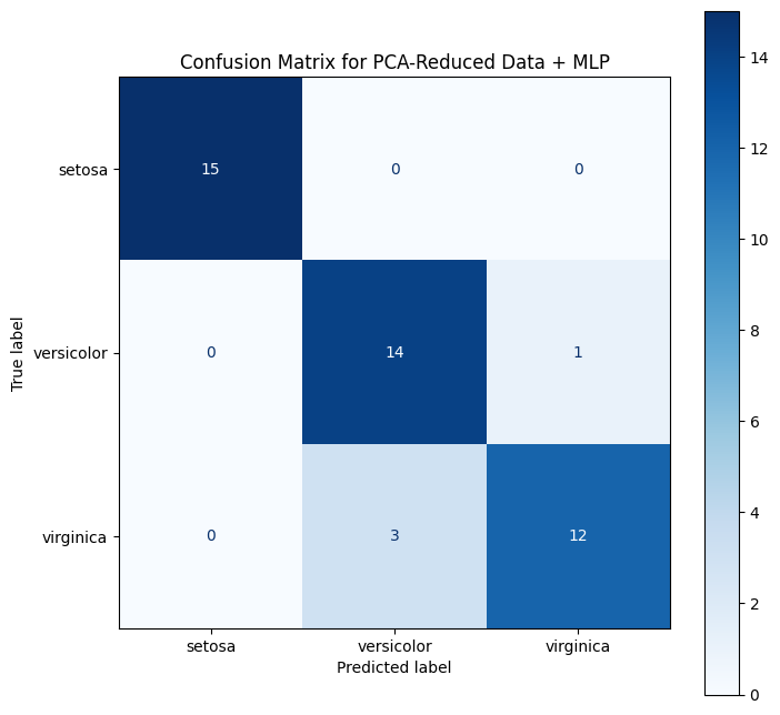
plt.title("Confusion Matrix for PCA-Reduced Data + MLP")
plt.show() # Display the plot
# -----------------------------------------
# --- EXPORT 1: Neural Network Model to ONNX ---
try:
# Requires: pip install skl2onnx onnx
from skl2onnx import convert_sklearn
from skl2onnx.common.data_types import FloatTensorType
# Define the input type: 2 input features (PC1, PC2) with float type
initial_type = [('float_input', FloatTensorType([None, 2]))]
# Export the MLP model
onnx_model = convert_sklearn(mlp, initial_types=initial_type, target_opset=13)
# Save to file
with open("iris_mlp.onnx", "wb") as f:
f.write(onnx_model.SerializeToString())
print("\n✅ Exported MLP model to ONNX format: 'iris_mlp.onnx'")
except ImportError:
print("\n⚠️ Skipping ONNX export: Install 'skl2onnx' and 'onnx' to enable this feature.")
# --- EXPORT 2: PCA Transformation to C Code using micromlgen ---
try:
# Requires: pip install micromlgen
from micromlgen import port
# Export the PCA object (which is a transformer) to C
c_code = port(pca, classmap={
0: 'SETOSA',
1: 'VERSICOLOR',
2: 'VIRGINICA'
})
# Save to C file (Note: using a standard local path)
with open('iris_pca_transform.c','w') as f:
f.write(c_code)
print("✅ Exported PCA transformation to C format: 'iris_pca_transform.c'")
except ImportError:
print("\n⚠️ Skipping C export: Install 'micromlgen' to enable this feature.")
Just for the sake of illustration, this is how the dataset looks like before applying the PCA:
And this is how it looks like after the PCA dimensionality reduction:
Explanation of the Neural Network
The MLPClassifier used here is configured as follows:
- Input Layer: Automatically set to 2 neurons, matching our two Principal Components (PC1 and PC2).
- Hidden Layer: A single layer with 10 neurons (hidden_layer_sizes=(10,)). This is a small, efficient size for an embedded device.
- Activation Function: ReLU (activation=’relu’). This non-linear function is computationally light and is the standard for modern NNs.
- Output Layer: Automatically set to 3 neurons (for the three Iris species) with a softmax activation implicitly handled by the classifier for multi-class problems.
This simple 2-10-3 architecture is much more representative of the type of model that would be converted to TFLite and deployed to an STM32.
The goal is not to achieve the best in class classifier, so no real effort was used to achieve higher accuracy. As is, this classifier, after PCA, achieved around 91% accuracy, with the following Confusion Matrix:
Once the model is to your liking, you can export the content using the ONNX framework, which is compatible with X-Cube-AI.
5. X-Cube-AI Cloud Deployment
STMicroelectronics’ X-CUBE-AI is an expansion package for the STM32CubeMX environment that optimizes and deploys trained ML models (including those from frameworks like scikit-learn, TensorFlow, and PyTorch) onto STM32 microcontrollers.
- Model Conversion and Optimization: X-CUBE-AI converts the trained model (e.g., a TFLite file or a scikit-learn pipeline) into highly optimized, platform-independent C code tailored for the target STM32 device.
- Analysis and Profiling: The tool provides detailed reports on the model’s memory footprint (Flash/RAM) and estimated execution time, which is critical for selecting the right microcontroller and ensuring real-time performance.
- Support for ML Algorithms: It supports not only Neural Networks but also classic ML algorithms, making it suitable for deploying a PCA-reduced classifier directly.
X-CUBE-AI simplifies the process of getting the Python-trained PCA + Classifier model onto the STM32, automatically managing the necessary C implementation of the mathematical operations.
To simplify even further, the Home – ST Edge AI Developer Cloud will be used instead of starting from the local CubeMX. Follow the steps below to evaluate the model behavior:
1. Sign in/Log in
2. Load your model using the “New Model” icon
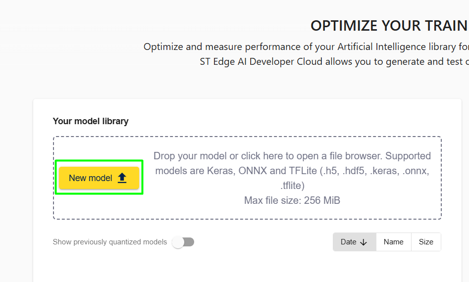
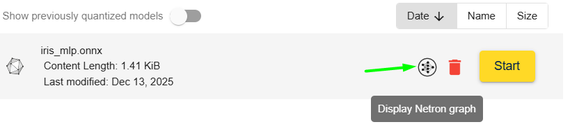
3. Click in Start to evaluate the model or in the Netron Graph to see your model
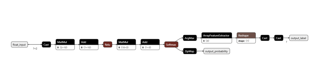
3.1 Model view:
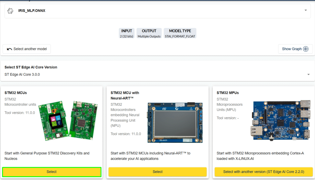
4. Select the board to used as test:
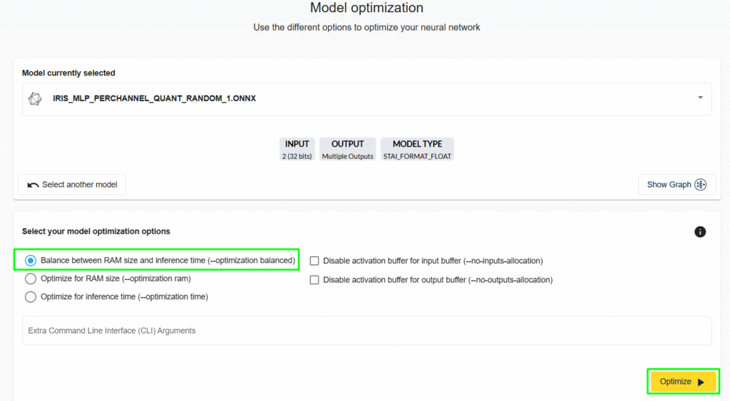
5. Launch Quantization or click “Go next”. Select the Model optimization:
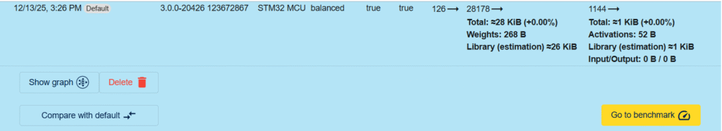
5.1 Check the model size:
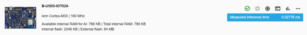
6. Go to benchmark and then select the desired board and click “Start Benchmark”. This shows the model’s inference time:
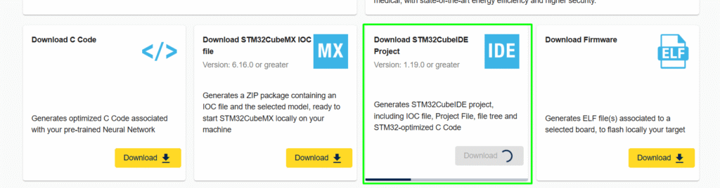
7. The last step is to generate the code/project:
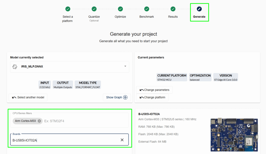
At the bottom of the page, select how the code/project should be generated:
6. Code validation
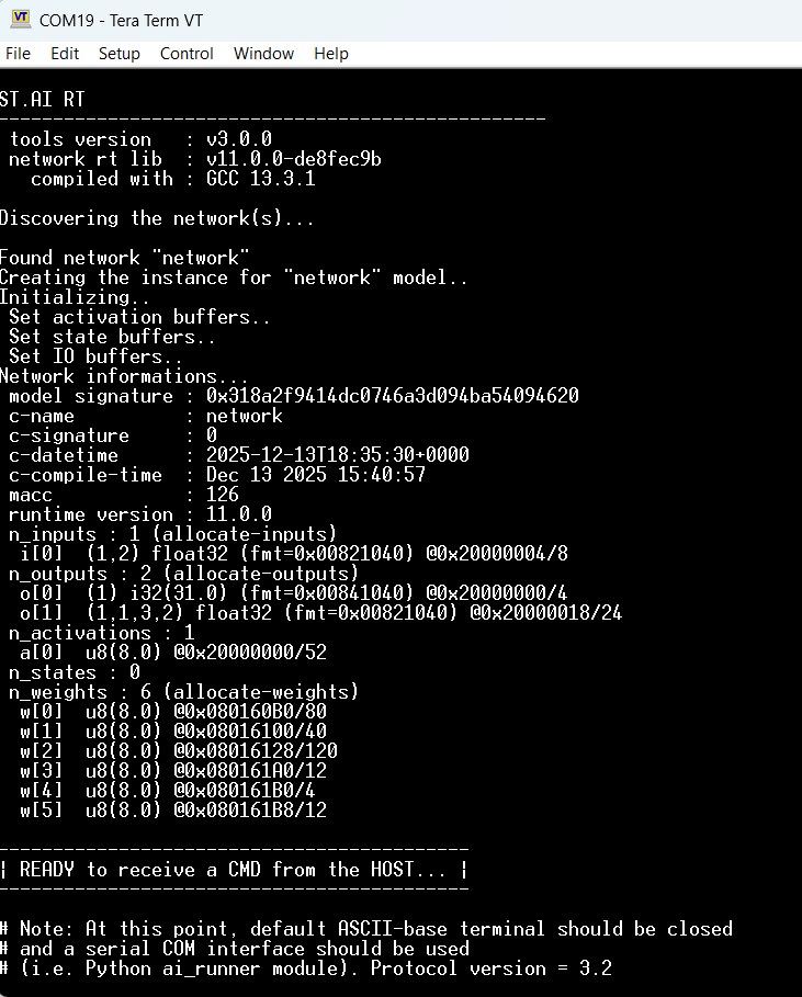
Open the created project, build it and load the code. On the terminal you’ll see the following boot up message:
From this point, follow the instructions in the article to create/customize the ai_runner: How to use the AiRunner package
If that is not the desired path, start from the *.ioc file, as shown in the other article: – Hacker Embedded TinyML Lab: Simple MLP for STM32 TinyML Deployment with X-Cube-AI
Remember to manually add the iris_pca_transform.c into your project, use the transform() function to apply the PCA before inserting the buffer into the AI model for real usage and not only model evaluation.
Minor final note, Note, the iris_pca_transform.c is actually created as a C++, so if the CubeIDE was made to use only C files, a minor conversion is needed, similar to this:
eloquent_ml_port_pca.h (Header File)
					#ifndef ELOQUENT_ML_PORT_PCA_H
#define ELOQUENT_ML_PORT_PCA_H

#include <stddef.h>
#include <stdint.h>

// Define the size constants
#define PCA_INPUT_SIZE 4
#define PCA_OUTPUT_SIZE 2

// Define the structure to hold the constant PCA transformation matrices
typedef struct {
    // Mean vector for standardization/scaling (all zeros in this example)
    const float mean[PCA_INPUT_SIZE];
    // Principal components (eigenvectors) matrix (2 components x 4 features)
    const float components[PCA_OUTPUT_SIZE][PCA_INPUT_SIZE];
} pca_transformer_t;

/**
 * Global PCA transformer instance initialized with the constants from the C++ code.
 */
extern const pca_transformer_t g_pca_transformer;

/**
 * @brief Computes the dot product of a data vector and a weight vector,
 * applying the mean correction first.
 *
 * @param x The input data vector (PCA_INPUT_SIZE elements).
 * @param mean_vec The mean vector to subtract.
 * @param weights The weight vector (Principal Component coefficients).
 * @return float The result of the dot product.
 */
float pca_dot_product(const float *x, const float *mean_vec, const float *weights);

/**
 * @brief Apply dimensionality reduction using PCA.
 *
 * @param x The input vector (4 elements) to transform.
 * @param dest The destination vector (2 elements) to store the result.
 * If NULL, the result cannot be stored.
 */
void pca_transform(const float *x, float *dest);

#endif // ELOQUENT_ML_PORT_PCA_H
eloquent_ml_port_pca.c (Source File)
					#include "eloquent_ml_port_pca.h"
#include <string.h> // For memcpy

// --- Constant Data Tables (equivalent to hardcoded values in C++ dot calls) ---

// NOTE: Since the C++ code used static float mean[] = { 0.0, 0.0, 0.0, 0.0 };
// and passed weights via varargs, we define the weights explicitly here.

const pca_transformer_t g_pca_transformer = {
    // mean (used for standardization, all zeros in the original code)
    .mean = { -0.0, -0.0, -0.0, -0.0 },

    // components (Principal Component vectors/eigenvectors)
    // Row 0: PC1 weights
    // Row 1: PC2 weights
    .components = {
        { 0.52106591467f, -0.269347442506f, 0.580413095796f, 0.564856535779f }, // PC1
        { 0.377417615565f, 0.923295659541f, 0.024491609086f, 0.066941986968f }  // PC2
    }
};

/**
 * @brief Computes the dot product of a data vector and a weight vector,
 * applying the mean correction first.
 */
float pca_dot_product(const float *x, const float *mean_vec, const float *weights) {
    float dot_result = 0.0f;
    for (uint16_t i = 0; i < PCA_INPUT_SIZE; i++) {
        // (x[i] - mean[i]) * weights[i]
        dot_result += (x[i] - mean_vec[i]) * weights[i];
    }
    return dot_result;
}


/**
 * @brief Apply dimensionality reduction using PCA.
 */
void pca_transform(const float *x, float *dest) {
    // Ensure destination pointer is valid
    if (dest == NULL) {
        return; // Cannot proceed if dest is NULL in pure C without modifying x
    }

    // Calculate the two principal components
    // PC1 = dot(x, PC1_weights)
    dest[0] = pca_dot_product(x, g_pca_transformer.mean, g_pca_transformer.components[0]);

    // PC2 = dot(x, PC2_weights)
    dest[1] = pca_dot_product(x, g_pca_transformer.mean, g_pca_transformer.components[1]);

    // NOTE: The original C++ code had a special check to overwrite 'x' if 'dest' was NULL.
    // In clean C, we avoid modifying 'x' if 'dest' is NULL, and require 'dest' to be allocated by the caller.
    // The C++ original: memcpy(dest != NULL ? dest : x, u, sizeof(float) * 2);
    // This is implicitly handled by writing directly to 'dest[0]' and 'dest[1]' above.
}
7. Results
The Python code demonstrates that the first two principal components capture over 97% of the total variance in the Iris dataset. This dramatic reduction from 4 features to 2 allows the classifier to achieve a high accuracy (typically around 95-98% depending on the train/test split) while operating on a vector that is half the original size. On an STM32, this smaller data size and simpler model directly translate to ultra-low-power, fast inference suitable for battery-powered edge devices.
Conclusion
PCA is an invaluable preprocessing step for deploying machine learning models to memory and power-constrained STM32 microcontrollers. By effectively reducing the dimensionality of the input data, it significantly lowers the complexity and resource demands of the subsequent classification model. Combined with tools like TFLite Micro or the highly optimized X-CUBE-AI, PCA enables the deployment of powerful, accurate ML solutions to the very edge of the network.