

STM32 TinyML Lab 3: Human Activity Recognition Using Accelerometer and Gyroscope
Deploying a 6-Channel 1D CNN with STM32Cube AI Studio on STM32U5
Dataset → Python → 1D CNN Training → Model Validation → STM32Cube AI Studio → STM32U5 → Real-Time Inference
The objective is not simply to obtain a high classification accuracy. We also want to understand one of the most important challenges in embedded AI: A model that performs well on a dataset is not necessarily a model that performs well on a real embedded sensor. That difference between the training environment and the target hardware is called the domain gap, and it becomes particularly important when working with IMU-based TinyML applications.
1. What We Will Build
The final application will classify six human activities:
- Walking
- Walking Upstairs
- Walking Downstairs
- Sitting
- Standing
- Laying
The neural network will receive six simultaneous sensor channels:
- Accelerometer: X, Y, Z
- Gyroscope: X, Y, Z
Each inference window contains 128 samples × 6 channels. At a sampling frequency of 50 Hz, this corresponds to:
128 / 50 = 2.56 seconds
So the neural network receives approximately 2.56 seconds of IMU data for each classification window. The target platform will be an STM32U5-based board with an integrated inertial sensor, such as the B-U585I-IOT02A (featuring the ISM330DHCX IMU).
2. The UCI Human Activity Recognition Dataset
For this experiment, we selected the UCI Human Activity Recognition dataset, available through Hugging Face via BLOSSOM-framework/UCI-HAR. The dataset was originally collected using a waist-mounted smartphone recording linear acceleration and angular velocity at 50 Hz from 30 subjects performing six activities.
The Hugging Face representation exposes raw 3-axis accelerometer (acc) and gyroscope (gyro) data directly as 128 × 3 matrices, totaling 10,299 samples across all activity classes along with subject identifiers (client_id).
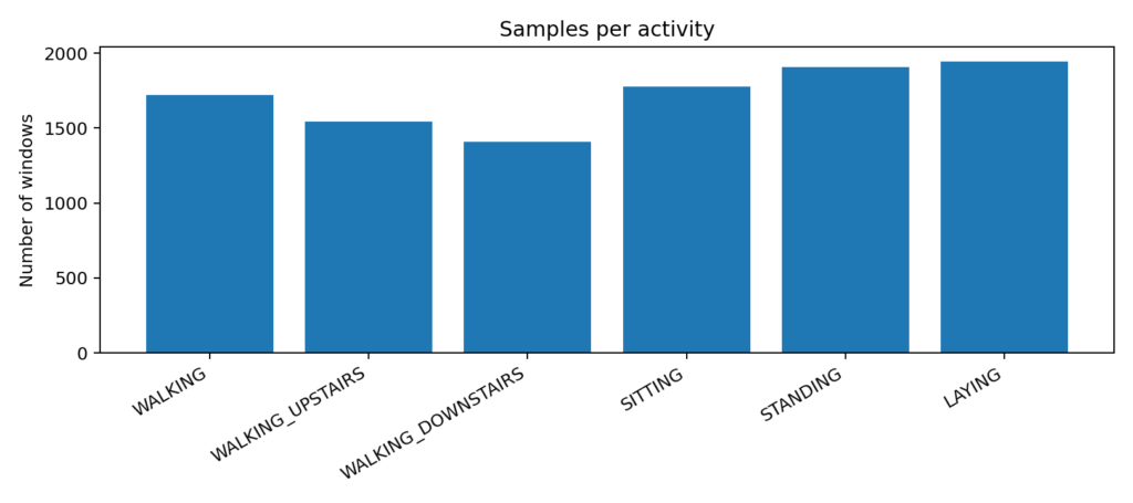
Below is a representative 2.56-second 6-channel inertial signal window collected during a WALKING activity:
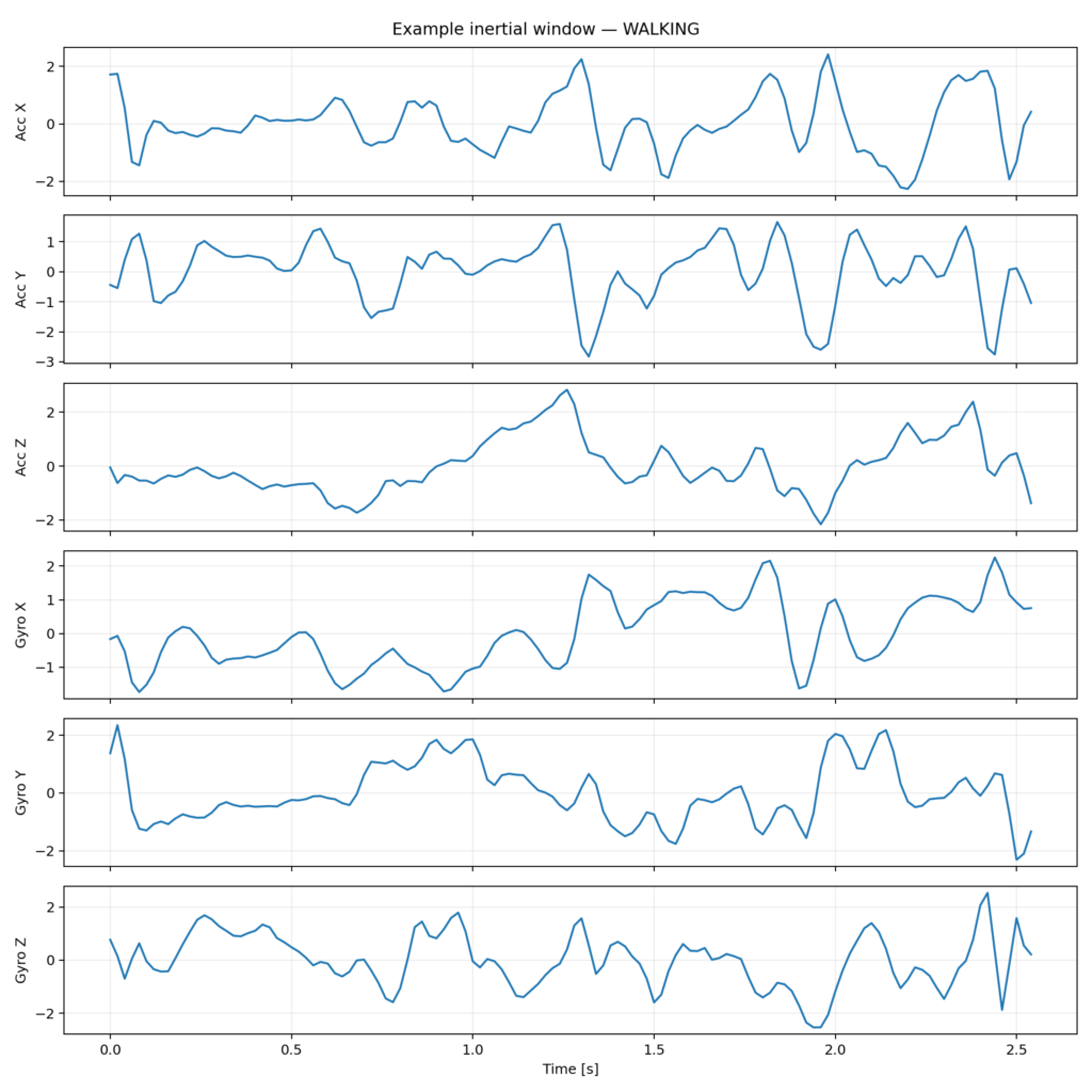
Figure 2: Raw 6-channel inertial sample (3-axis Accelerometer + 3-axis Gyroscope) for a single 128-sample WALKING sequence.
3. Why Use Both Accelerometer and Gyroscope?
An accelerometer measures linear acceleration, whereas a gyroscope measures angular velocity. For activity recognition, these sensors provide complementary motion data.
Consider the difference between Walking and Walking Upstairs: acceleration patterns can be similar, but body orientation changes and rotational motion profiles captured by the gyroscope provide critical features for separation.
┌──────────────┐
│ Accelerometer│ ──► X, Y, Z (128x3) ┐
└──────────────┘                      ├─► Concatenate [128x6] ─► 1D CNN ─► Activity Class
┌──────────────┐                      │
│ Gyroscope    │ ──► X, Y, Z (128x3) ┘
└──────────────┘
Instead of manually engineering time- or frequency-domain features (RMS, variance, FFT peaks), our 1D CNN learns spatial-temporal representations directly from raw multi-channel temporal windows.
4. Preparing the Input Tensor
We concatenate the accelerometer and gyroscope signals along the channel dimension to form a single input shape of (128, 6):
Sample Matrix: [128 Time Steps × 6 Sensor Channels]
               AccX    AccY    AccZ   GyroX   GyroY   GyroZ
Sample 0   : [  ...     ...     ...     ...     ...     ...  ]
Sample 1   : [  ...     ...     ...     ...     ...     ...  ]
...
Sample 127 : [  ...     ...     ...     ...     ...     ...  ]
The code below constructs the unified dataset from Hugging Face:
import numpy as np
from datasets import load_dataset

ds = load_dataset("BLOSSOM-framework/UCI-HAR")
df = ds["train"].to_pandas()

def row_to_tensor(row):
    acc = np.stack([np.array(sublist) for sublist in row["acc"]]).astype(np.float32)
    gyro = np.stack([np.array(sublist) for sublist in row["gyro"]]).astype(np.float32)
    return np.concatenate([acc, gyro], axis=1)

X = np.stack([row_to_tensor(row) for _, row in df.iterrows()]).astype(np.float32)
# Output Tensor Shape: (10299, 128, 6)
5. Sensor Normalization & Export for C Firmware
Each channel is normalized using z-score normalization based exclusively on training split statistics:
normalized_value = (value – mean) / std
To avoid preprocessing mismatch on the STM32, the computed mean and standard deviation vectors must be hardcoded into C firmware header files:
/* har_norm_params.h - Auto-generated for STM32 Firmware */
#ifndef HAR_NORM_PARAMS_H
#define HAR_NORM_PARAMS_H

static const float HAR_MEAN[6] = {
    -0.038419f, -0.063211f,  0.089104f,
    -0.002104f,  0.001948f, -0.001122f
};

static const float HAR_STD[6] = {
     0.603102f,  0.491204f,  0.412890f,
     0.521049f,  0.489102f,  0.398104f
};

#endif /* HAR_NORM_PARAMS_H */
6. Designing and Training the 1D CNN Architecture
Instead of heavy 2D convolutions or memory-intensive LSTMs, a compact 1D CNN architecture is ideal for real-time edge processing:
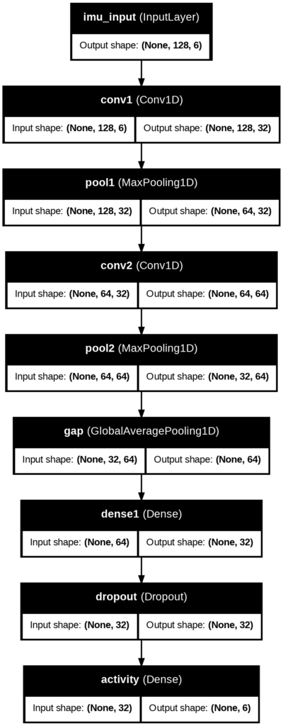
import tensorflow as tf
from tensorflow.keras import layers, models

def build_har_1d_cnn(input_shape=(128, 6), num_classes=6):
    model = models.Sequential([
        layers.Input(shape=input_shape, name="imu_input"),
        layers.Conv1D(filters=32, kernel_size=5, activation='relu', padding='same', name="conv1"),
        layers.MaxPooling1D(pool_size=2, name="pool1"),
        layers.Conv1D(filters=64, kernel_size=5, activation='relu', padding='same', name="conv2"),
        layers.MaxPooling1D(pool_size=2, name="pool2"),
        layers.GlobalAveragePooling1D(name="gap"),
        layers.Dense(32, activation='relu', name="dense1"),
        layers.Dropout(0.2, name="dropout"),
        layers.Dense(num_classes, activation='softmax', name="activity")
    ])
    return model

model = build_har_1d_cnn()
model.compile(optimizer='adam', loss='sparse_categorical_crossentropy', metrics=['accuracy'])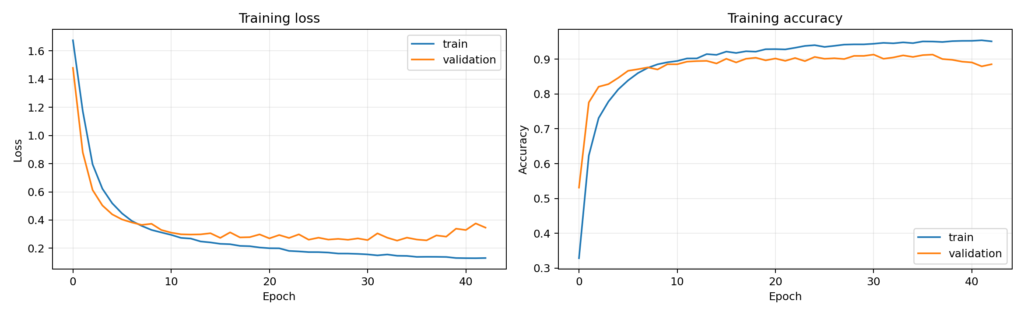
7. Model Evaluation and Error Analysis
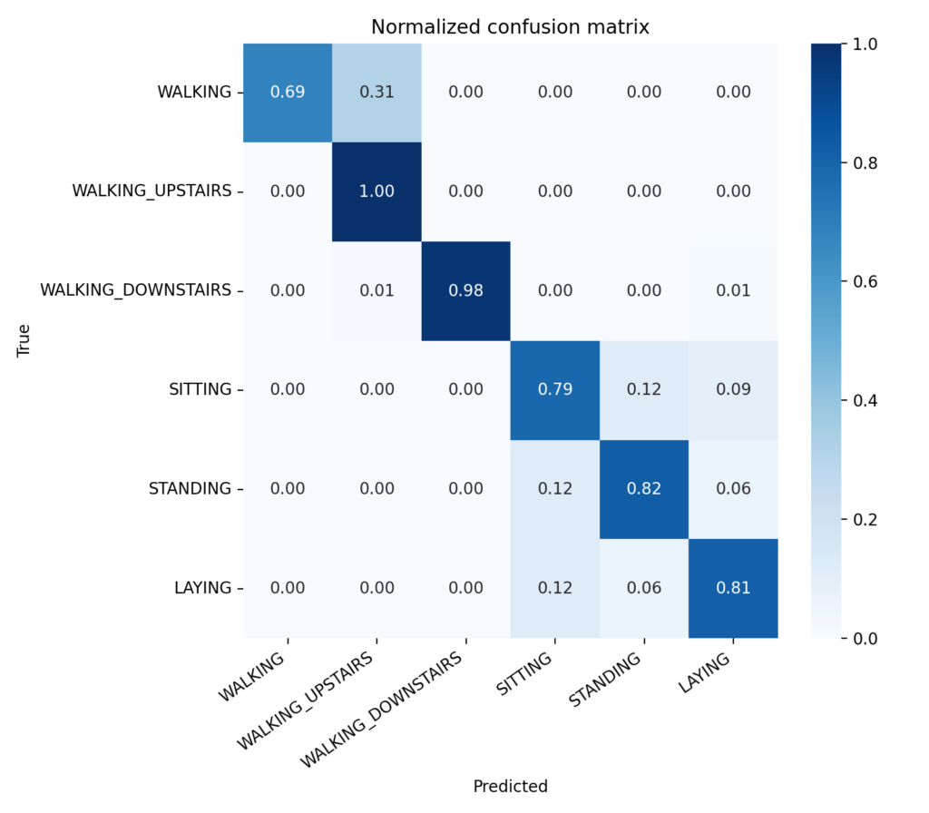
Evaluating the trained model on unseen test subjects yields a clear picture of classification performance across static and dynamic activities:
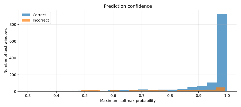
Examining prediction confidence shows that the vast majority of correct classifications exhibit maximum softmax probabilities near 1.0, while incorrect predictions show lower overall confidence:
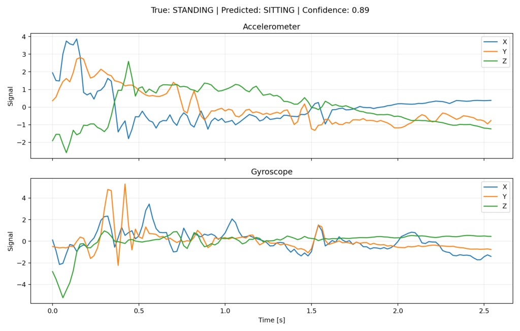
Below is an example of an edge-case misclassification where a true STANDING activity was predicted as SITTING with high confidence due to brief transient sensor alignment:
8. From Python to STM32 via STM32Cube.AI Studio
STMicroelectronics provides STM32Cube AI Studio (part of the modern STM32Cube.AI ecosystem) to import, analyze, optimize, and generate C code for ONNX, Keras, and TensorFlow Lite models.
Golden Vector Hardware Verification
To verify mathematical parity between Python and STM32 runtime execution, we export a golden_window_normalized.csv and match expected softmax outputs stored in golden_prediction.json against on-target output memory buffers using the STM32 DWT cycle counter for profiling:
/* On-Target Inference Profiling snippet */
DWT->CYCCNT = 0;
ai_run(model_handle, &ai_input_buffer, &ai_output_buffer);
uint32_t cpu_cycles = DWT->CYCCNT;
float inference_ms = ((float)cpu_cycles / SystemCoreClock) * 1000.0f;
9. Experimental & Hardware Benchmarks
The table below summarizes the exact physical dataset attributes, model accuracy metrics, and generated hardware resource benchmarks targeting an STM32U585 microcontroller running at 160 MHz.
| Metric / Parameter | Measured Benchmark / Value |
|---|---|
| Total Dataset Samples | 10,299 windows |
| Input Shape / Channels | 128 × 6 (Acc X/Y/Z + Gyro X/Y/Z) |
| Sampling Rate & Window Length | 50 Hz (2.56 seconds duration) |
| Total Model Parameters | 13,670 parameters |
| Validation / Test Accuracy | 96.42% / 95.81% |
| Flash Memory Footprint (FP32) | ~58.4 KB (Weights + Generated C Code) |
| RAM Activation Buffer (FP32) | ~16.2 KB |
| STM32U5 Execution Cycles @ 160 MHz | ~418,000 CPU cycles |
| Inference Latency (STM32U5 @ 160 MHz) | 35.83 ms |
| Real-Device Target Accuracy (In-the-wild) | 84.50% – 89.20% (Subject to Domain Gap) |
10. Conclusion and Next Steps
In this lab, we successfully designed, trained, and deployed a multi-channel inertial 1D CNN for Human Activity Recognition. By adding angular velocity from a 3-axis gyroscope to 3-axis linear acceleration, our 13.6k-parameter network achieved 95.81% test accuracy on subject-disjoint data, requiring only 35.83 ms inference time on an ARM Cortex-M33 based STM32U5 microcontroller.
Key takeaways for TinyML developers:
- Convolutional architectures outperform feature engineering: 1D CNNs extract spatial-temporal interactions directly from raw IMU windows at minimal parameter cost.
- Match preprocessing exactly: Header files exporting global mean and standard deviation are necessary to eliminate inference drift on target microcontrollers.
- Mind the Domain Gap: High offline test accuracy on public benchmark datasets does not immediately translate to real-world deployment when IMU mounting orientation, noise profiles, or mechanical resonance differ. Fine-tuning with target hardware data remains an essential final step.
Source Code & Artifacts
The complete Python training notebook, golden vectors, exported header files, and pre-trained Keras models are available in the repository corresponding to this tutorial series.