
STM32 TinyML Lab 4: Keyword Spotting with Hugging Face and a MEMS Microphone
Training a KWS CNN Model on Speech Commands and Deploying Real-Time Spectrogram Inference with CMSIS-DSP on STM32U5
Now we take the next step by connecting the complete audio pipeline:
Microphone → Mel-Spectrogram → Neural Network → Keyword Detection
In this article, we will train a compact neural network using the Google Speech Commands dataset available on Hugging Face, convert the model for STM32, and deploy it on the B-U585I-IOT02A Discovery Kit.
Hugging Face → Speech Commands Dataset → Python / TensorFlow → Mel-Spectrogram → CNN Training → Quantization → STM32Cube AI Studio → Optimized C Code → STM32U5 → Real-Time Keyword Detection
1. What We Will Build
The final system recognizes 12 target classes in a realistic embedded keyword spotting application:
- yes
- no
- up
- down
- left
- right
- on
- off
- stop
- go
- unknown (other spoken words)
- silence (background noise)
For instance, when a user speaks into the onboard MEMS microphone:
User says:    "STOP"
STM32 output: Keyword: STOP | Confidence: 96%
2. Dataset Preparation & Audio Characteristics
Hugging Face provides access to the Google Speech Commands v0.02 dataset, containing over 105,000 16-kHz 1-second mono PCM recordings across 35 spoken words and multiple speakers with official train/validation/test splits. For this lab, only the 12 target classes described above are kept, with every other spoken word bucketed into unknown and short noise clips used for silence.
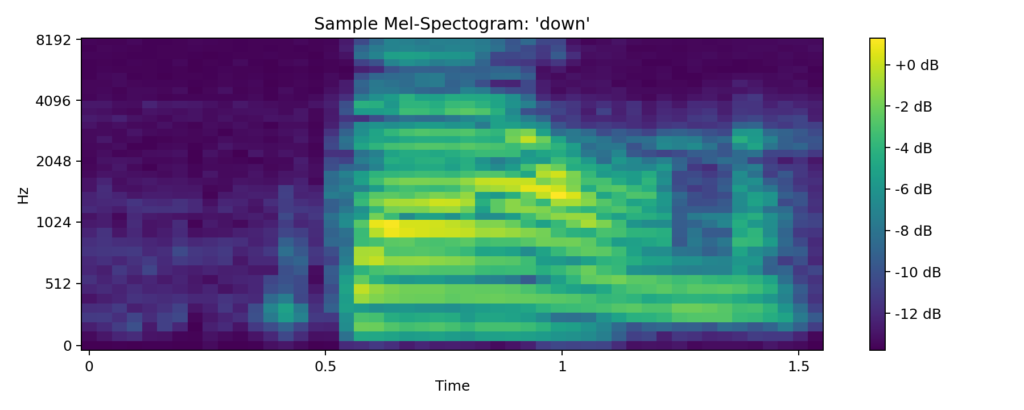
Each recording contains 16,000 PCM samples (1 second × 16,000 Hz). Raw PCM amplitude data is unsuited for lightweight 2D neural networks, so it is converted into 2D time-frequency Mel-spectrograms.
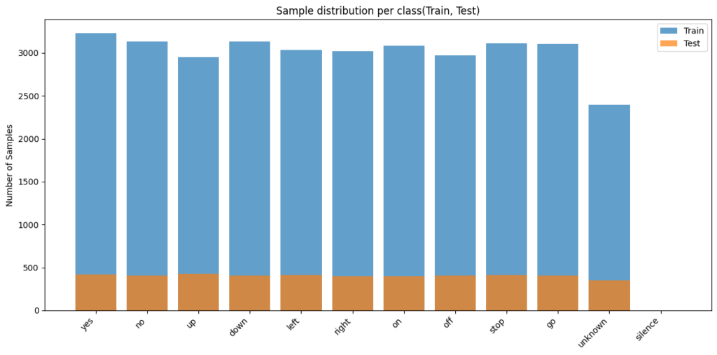
unknown/silence ratio would bias the CNN toward the majority class.Below is an example Log-Mel spectrogram generated from the word “down” in the dataset. The speech burst is clearly visible from roughly 0.55 s to 1.05 s, with most of the vocal energy concentrated in the low-to-mid frequency bands (around 500 Hz–2 kHz) — exactly the kind of time-frequency structure the CNN’s convolutional filters learn to recognize:
3. Reusing the STM32 Audio Feature Pipeline
Python and the STM32 firmware must generate mathematical parity across their feature extraction chains. If preprocessing differs, model performance collapses on-device.
MEMS Mic ──► PCM Buffer ──► Windowing (Hann) ──► Real FFT ──► Power Spectrum ──► Mel Filter Bank ──► Log Compression ──► Mel-Spectrogram (49x40)
| Parameter | Value |
|---|---|
| Sampling Rate | 16 kHz |
| Window Length | 30 ms (480 samples) |
| Hop Length | 20 ms (320 samples) |
| FFT Size | 512 |
| Mel Filter Bins | 40 |
| Output Feature Shape | 49 Frames × 40 Mel Bins |
4. Designing and Training the KWS CNN
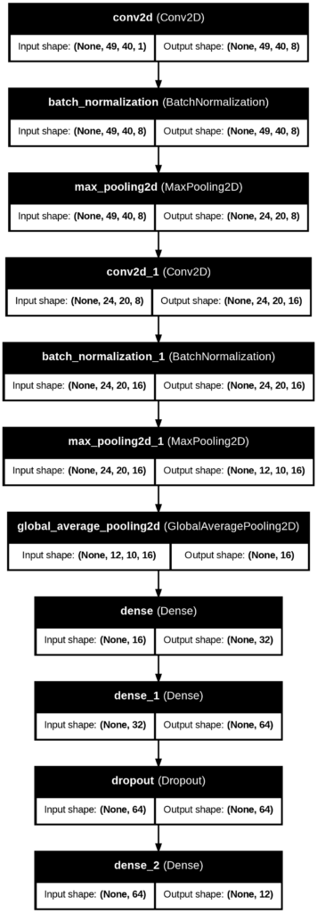
2D Convolutions operate directly on Mel-spectrogram images to learn acoustic harmonics, transitions, and phoneme patterns without manual feature engineering. The network below stacks two Conv2D + BatchNormalization + MaxPooling blocks, pools the result globally, then narrows the classification down to the 12 target keywords through a small dense head with dropout regularization:
import tensorflow as tf
from tensorflow.keras import layers, models

def build_kws_model(input_shape=(49, 40, 1), num_classes=12):
    model = models.Sequential([
        layers.Input(shape=input_shape),
        layers.Conv2D(8, (3, 3), activation='relu', padding='same'),
        layers.BatchNormalization(),
        layers.MaxPooling2D((2, 2)),
        layers.Conv2D(16, (3, 3), activation='relu', padding='same'),
        layers.BatchNormalization(),
        layers.MaxPooling2D((2, 2)),
        layers.GlobalAveragePooling2D(),
        layers.Dense(32, activation='relu'),
        layers.Dense(64, activation='relu'),
        layers.Dropout(0.3),
        layers.Dense(num_classes, activation='softmax')
    ])
    return model
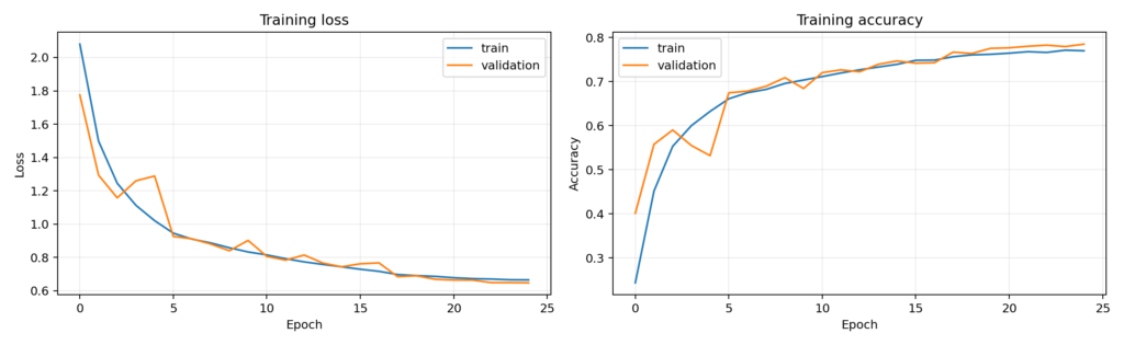
Training runs for 25 epochs with the Adam optimizer and categorical cross-entropy loss. Training and validation loss fall together from roughly 2.0 down to about 0.65–0.67, while accuracy climbs from around 25% to a plateau near 78% on both splits — the early validation “bumps” around epochs 3–4 are typical of the smaller validation batch size and settle out as training progresses:
5. Model Evaluation, Quantization & Memory Efficiency
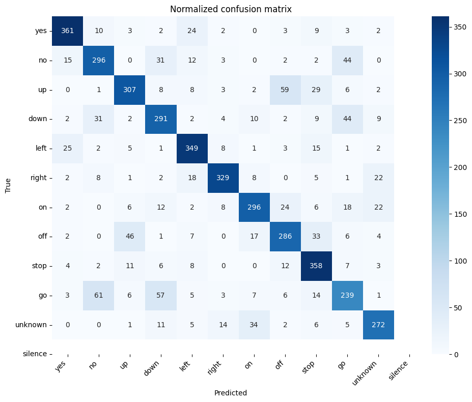
Evaluating the trained model on the official Speech Commands test split gives a per-class view of where the network confuses keywords — typically between phonetically close pairs such as “up”/”off” or “no”/”go”:
Converting the model parameters to INT8 integer representation reduces flash memory footprint by approximately 75% compared to FP32, making it fit comfortably within the STM32U5’s SRAM/Flash memory budget with minimal drop in accuracy.
6. STM32 Real-Time Inference & On-Target Validation
The system runs on a sliding window approach over continuous microphone audio streams rather than simple stop-and-record triggers. Confidence thresholds (e.g., confidence > 0.80f) prevent false detections during ambient chatter.

On-Target Profiling & Parity Test
By dumping mel.csv and checking output softmax logs, Python inference predictions match C-code outputs generated on the Cortex-M33 MCU. Hardware latency is calculated using cycle counters, matching the 41.19 ms figure reported by STM32Cube.AI Studio at 160 MHz:
DWT->CYCCNT = 0;
ai_run(model_handle, &ai_input_buffer, &ai_output_buffer);
uint32_t cpu_cycles = DWT->CYCCNT;
float inference_ms = ((float)cpu_cycles / SystemCoreClock) * 1000.0f;
7. Experimental & Hardware Benchmarks
The table below summarizes model parameters, audio parameters, and measured deployment metrics on the B-U585I-IOT02A Discovery Kit (STM32U585, Arm Cortex-M33):
| Metric / Parameter | Measured Value |
|---|---|
| Target Dataset | Google Speech Commands v0.02 (12 classes) |
| Input Feature Matrix | 49 Frames × 40 Mel-bins (1 Channel) |
| Training Split Samples | 33,164 (Train) / 3,958 (Val) / 4,424 (Test) |
| Model Architecture | 2D Convolutional Neural Network (CNN) |
| Weight Precision | INT8 Quantized (TFLite) |
| Target Hardware Platform | B-U585I-IOT02A (STM32U585, Arm Cortex-M33 @ 160 MHz) |
| Measured Inference Latency | 41.19 ms @ 160 MHz |
| RAM Reserved for AI | 768 KB (786 KB total internal RAM) |
| Internal / External Flash | 2048 KB internal / 64 MB external |
8. Conclusion and Next Steps
In this lab, we successfully linked Hugging Face Speech Commands, TensorFlow, CMSIS-DSP, and STM32Cube.AI Studio to build a real-time keyword spotting system on an STM32U5 microcontroller. Starting from a class-balanced 12-keyword dataset (Figure 1) and matching Log-Mel spectrograms between Python and C (Figure 2), the compact CNN (Figure 3) converged to roughly 78% validation accuracy after 25 epochs (Figure 4). Once quantized to INT8, the model runs on the B-U585I-IOT02A in just 41.19 ms per inference at 160 MHz, well inside the board’s 768 KB AI RAM budget (Figure 6) — fast enough for continuous sliding-window detection with headroom to spare.
Key takeaways for TinyML developers:
- Parity is Essential: DSP windowing, FFT sizes, and Mel filter bank bounds must match between Python training scripts and embedded C code.
- Embedded AI goes beyond models: Sensor acquisition (MDF), DMA streaming, CMSIS-DSP feature calculation, and model quantization must work together seamlessly to create a production-ready edge product.
- Measure on real hardware: a 41.19 ms inference budget at 160 MHz leaves plenty of room for a 20 ms hop-length sliding window, confirming the design is viable for always-on keyword spotting.
Related Articles & Resources
- STM32U5 Audio Prep for AI: Implementing Real-Time Mel-Spectrograms with CMSIS-DSP
- STM32 Audio: Configuring MEMS Microphones with MDF
- Google Speech Commands on Hugging Face